Understanding Recursion

Rather than using the popular joke about recursion (see bottom), I’ll reference a very peculiar adage which makes use of this particular mental model:

The Hogstadter’s Law, states that:

It always takes longer than you expect, even when you take into account Hofstadter’s Law.

See what happened there? The law is a self-referential adage, that tries to describe the widely experienced difficulty of accuratelly estimate the time it will take to complete tasks of substancial complexity.

I feel it describes very much my past experience trying to objectively explain the time and budget constrains in a software project where the requirements keep changing. That should be called the Oschvr’s Law

Anyway, back to topic.

Definition#

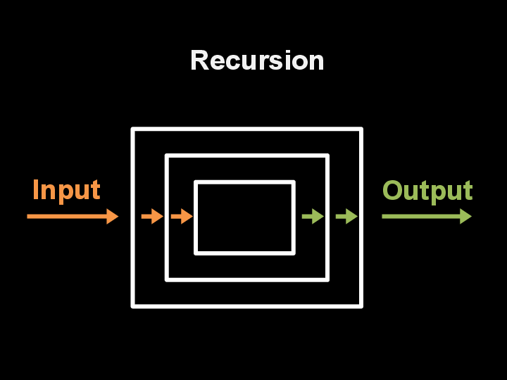
Recursion is the process of solving a problem by dividing it into smaller version of the problem.

By this definition, whenever the division of a given problem is small enough, it will reach a “base case”, or when the problem can be solved directly.

Amazing right? A problem’s solution that calls itself to solve the problem !

Rationale#

Why do we need recursion? Can’t we just use a loop and get over it?

The answer is … it depends

The fact is that mathematically, it makes more sense to use a recursive solution for most problems and for sufficiently large inputs of those problems.

But there will be sometimes where iterative solutions make way more sense when the problem tends to be complicated, harder to analyse and generally less efficient with recursion.

For now, let’s look at some examples of recursive implementations to clarify the concept.

Example: Substraction#

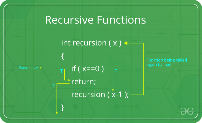
Let’s look at a more hands on example in pseudocode:

We have:

• A function definition
• A base case
• A call to the same function

This function will substract 1 to x, recursively until we reach the base case 0. Here’s implemented in Go

func main() {
        // We want to go from 10 to 0
	fmt.Println(recursion(10))
}

func recursion(x int) int {
	if x == 0 {
		return 0
	}
	fmt.Print(x, ", ")
	return recursion(x - 1)
}

This will output:

10, 9, 8, 7, 6, 5, 4, 3, 2, 1, 0

Let’s look at another example.

Example: Factorial#

Factorials are very useful in many areas of mathematics and computer science. Given that:

A Factorial number is the product of every whole number from 1 to n

For example if n = 3, then 3! = 3 x 2 x 1 = 6

This is another excellent case where we can apply a recursive algorithm to calculate the result.

In pseudocode we will define our function, our base case and our recursive call.

// function definition
int factorial(n)

  // base case
  if (n == 0) {
    return 1
  }

  // recursive call
  n * factorial(n - 1)

Here’s converted go Go, in order to test it:

func main() {
	fmt.Println(factorial(10))
}

func factorial(n int) int {
	if n == 0 {
		return 1
	}
	return n * factorial(n-1)
}

The output is:

3628800 in 38.27µs

Example: Fibonacci#

The Fibbonacci sequence implementation is a very popular example of a recursive procedure. The formal definition states:

$If n >= 1$

$F(n) = F(n-1) + F(n-2)$

Here’s the recursive implementation in Go

func main() {
	start := time.Now()
	n := 10
	fmt.Println(fibonacci(n))
	fmt.Println(time.Since(start))

}

// Recursive fibonacci
// function definition
func fibonacci(n int) int {
	// Base case
	if n <= 1 {
		return n
	}
	// F(n) = F(n-1) + F(n-2)
	return fibonacci(n-1) + fibonacci(n-2)
}

The output is

55 In 49.64µs

Conclusion#

Recursion is one of the fundamental ideas behind Computer Science. Although is at first a hard concept to grasp, it can be understood with practice.

Many efficient algorithms of sorting and searching use recursion at the core to efficiently reduce the computational budget and get to the result faster.

In a following blog post, I will take a look on the computational analysis of recursive algorithms using Big O notation, and a couple of techniques and definitions.

Here’s the code repo with the examples above.

* In order to understand recursion, you must first understand recursion.